|
||
|
The power of a microarray experiment derives
from the identification of genes
differentially regulated across biological conditions.
To date, differential regulation is most often taken to mean
differential expression, and a number of useful methods for identifying
differentially expressed (DE) genes or gene sets
are available. However, such methods are not able to identify
many relevant classes of differentially regulated
genes. One important example concerns differentially co-expressed genes.
Choi and Kendziorski (2009) proposed an approach, gene set co-expression analysis (GSCA),
to identify differentially co-expressed gene sets.
The GSCA approach provides an FDR controlled list of
interesting gene sets, does not require that genes
be highly correlated in at least one biological condition,
and is readily applied to data from individual or multiple experiments, as we
demonstrate using data from studies of lung cancer and diabetes.
Details of the approach can be found in Choi and Kendziorski,
Bioinformatics 25(21): 2780-2786, 2009.
The GSCA package can be downloaded here,
which contains the R codes for running GSCA and an example data set used in Choi and Kendziorski (2009).
Codes and the data can also be loaded from this R image file.
Code for a brief example of a DC (Differential Co-expression) analysis with only 3 permutations is given here:
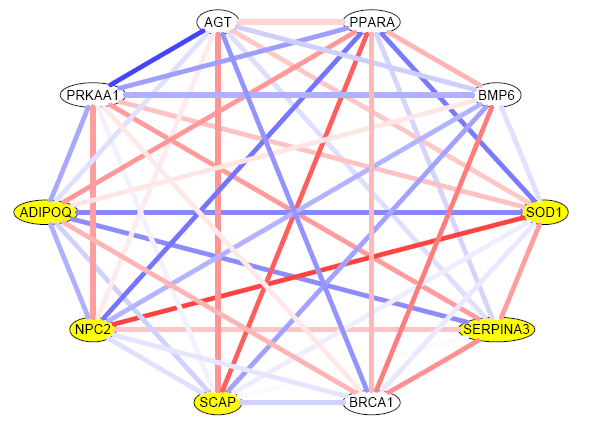
load("GSCA.RData") # if Windows, double-click the "GSCA.RData" icon. Once gene sets are identified as significantly DC between two groups, it is naturally of interest to visually display two condition-specific networks to contrast. The plot below is a normal-specific network from the Michigan lung cancer study, followed by the R code used to draw such a plot. Each edge is colored so it corresponds to the gene-gene pairwise Pearson correlation, with correlation values ranging from -1 to 1 are shown in blue to red. Yellow nodes are shown to indicate hypothetical DE genes in this example.
library(gplots) # for bluered() More detailed examples are available in the package vignette; further information is available in the manual.
Last Modified June 2009 |